Text Processing and Feature Extraction for Quantitative Text Analysis
Python User Group Workshop
Markus Konrad markus.konrad@wzb.eu
June 2017
Outline
- Introduction
- Text preprocessing
- Text tokenization
- Text normalization
- Text parsing and filtering
- Feature Extraction
- Bag-of-Words model
- tf-idf model
Introduction
Text analysis pipeline:
Collected text files → processed/normalized text data → extracted features → model
Book: D. Sarkar, Text Analytics with Python (apress 2016)
Please note: The code examples are only provided to show the basic concepts. You should use the recommended Python packages for real applications!
Text preprocessing
Goal: Transform raw text input into normalized sequence of tokens. Prepare for feature extraction.
"Hi. This is an example sentence in an Example Document." → [hi, example, sentence, example, document] → [1, 2, 1, 1]
Text processing includes many steps and hence many decisions that have big effect on your results. Several possibilities will be shown here. If and how to apply them depends heavily on your data and your later analysis.
The document corpus
A corpus contains the documents that we want to process. Each document can be accessed by a unique document label or document ID. The document itself is usually a (very long) character string (Python type: str) that may contain line breaks.
You normally load a corpus from files, a database or other sources.
# a small toy corpus with some (adapted) German newspaper headlines from June 20th
corpus = {   # document label: document text
    'spon1': 'Mehr Zustimmung zur EU auch wegen Trump – Danke May, danke Trump',
    'spon2': 'Nach Tod von US-Student Warmbier: Trump beschuldigt Nordkorea',
    'focus': 'Tod von US-Student Warmbier – Trump beschuldigt Nordkorea-Regime',
    'xyz': 'EU bleibt EU, aber EU-US-Beziehungen unter Trump weiter angespannt',   # stupid made up headline
}
# access by document label
corpus['spon1']
Tokenization
Goal: Break down document text into smaller, meaningful components (paragraphs, sentences, words) → from a document, form a list of tokens
In our case: We apply word tokenization, so token = word
With plain Python: calling split() on a string splits it by whitespace:
print(corpus['xyz'].split())
print(corpus['spon2'].split())
Tokenization is not trivial.
- how to handle punctuation, quotes, hyphens?
- how to handle contractions? ("don't" or "wasn't")
→ depends on your text (language, source/medium)
str.split()might not be optimal- NLTK implements several word- and sentence tokenizers, e.g.:
- TreebankWordTokenizer: Default tokenizer → punctuation become separate tokens
- RegExpTokenizer: Define your own tokenizer with Regular Expression rules
import nltk

# word_tokenize uses TreebankWordTokenizer by default
# set language to "german" to use German punctuation
print(nltk.word_tokenize(corpus['spon2'], language="german"))
nltk.word_tokenize("I wasn't there.") # default language is English
# tokenize whole corpus
tokens = {doc_label: nltk.word_tokenize(text, language="german")
          for doc_label, text in corpus.items()}
tokens.keys()
print(tokens['spon1'])
Text normalization
Can involve:
- expanding contractions
- expanding hyphenated compound words
- removing special characters
- case conversion
- removing stopwords
- correct spelling
- stemming / lemmatization
The order is important!
Expanding contractions
- strategy: make list of all possible contractions and their expanded replacement
- search & replace with Python using regular expressions
- not relevant here
- see "correct spelling" later
Expanding hyphenated compound words
- how to handle words like "US-Student"?
- leave as is
- strip hyphens (see "removing special characters" later)
- split by hyphens
# example to split by hyphen
split_tokens = []
for t in tokens['focus']:
    split_tokens.extend(t.split('-'))
print(split_tokens)
Problem: Would also split "e-mail" → ["e", "mail"]!
Removing special characters
- decide which special characters are not of interest → list of special characters that should be removed
- decision: remove any special characters in tokens/words ("US-Student" → "USStudent") or only sole characters?
- big effect on later steps, especially Part-of-Speech tagging!
Several ways, e.g. with regular expressions or str.translate:
import string
string.punctuation
del_chars = str.maketrans('', '', string.punctuation + '–')   # add another character "–"
print([t.translate(del_chars) for t in tokens['focus']])   # apply table "del_chars"
Our strategy: Split only if first compound word is possibly longer than one character.
def expand_compound_token(t, split_chars="-"):
    parts = []
    add = False   # signals if current part should be appended to previous part
    for p in t.split(split_chars):  # for each part p in compound token t
        if not p: continue  # skip empty part
        if add and parts:   # append current part p to previous part
            parts[-1] += p
        else:               # add p as separate token
            parts.append(p)
        add = len(p) <= 1   # if p only consists of a single character -> append the next p to it
        #add = p.isupper()   # alt. strategy: if p is all uppercase ("US", "E", etc.) -> append the next p to it

    return parts

print(expand_compound_token("US-Student"))
print(expand_compound_token("Nordkorea-Regime"))
print(expand_compound_token("E-Mail-Provider"))
tmp_tokens = {}
for doc_label, doc_tok in tokens.items():
    tmp_tokens[doc_label] = []
    for t in doc_tok:
        t_parts = expand_compound_token(t)
        tmp_tokens[doc_label].extend(t_parts)

print('Old:', tokens['focus'])
print('New:', tmp_tokens['focus'])
tokens = tmp_tokens
Case conversion
Usually: convert all words to lowercase.
Can be problematic because of "capitonyms":
- e.g. in English: "May" ≠ "may", "Pole" ≠ "pole"
- or in German (much more frequent): "Morgen" ≠ "morgen", "Laut" ≠ "laut"
Proper Part-of-Speech tagging might not be possible afterwards!
Methods in Python: str.lower(), str.upper()
print([t.lower() for t in tokens['focus']])
Removing stopwords
Stopwords are words that are removed before doing further text analysis. Usually: Very common words for a certain language that transport little information.
Stopword list depends on:
- language
- your data / research scenario (filter out too common words)
- later text analysis method, e.g.:
- tf-idf automatically reduces importance of very common words (as opposed to Bag-of-Words)
- sentiment analysis: bad idea to have words like "not" in the stopword list!
NLTK has a list of stopwords for some languages:
print('English:', nltk.corpus.stopwords.words('english')[:5], '...')
print('German:', nltk.corpus.stopwords.words('german')[:5], '...')
# usage example (will remove "von" tokens):
stopwords = nltk.corpus.stopwords.words('german')
[t for t in tokens['focus'] if t.lower() not in stopwords]
Correct spelling
Depends on your data → especially necessary when working with social media data, surveys, etc.
Available packages for automatic spell correction:
- PyEnchant
- aspell-python
- pattern (
suggest()function)
NLTK implements several stemming algorithms:
PorterStemmer,LancasterStemmer(English only)SnowballStemmer(supports 13 languages)
stemmer = nltk.stem.LancasterStemmer()
stemmer.stem('employees')
stemmer = nltk.stem.SnowballStemmer('german')
print('Bücher →', stemmer.stem("Bücher"))
print('gebuchte →', stemmer.stem("gebuchte"))
print('sahen →', stemmer.stem("sahen"))
Lemmatization
Find lemma (dictionary form) of a inflected word → a lemma is always a lexicographically correct word
Implemented for English in NLTK with WordNetLemmatizer.
lemmatizer = nltk.stem.WordNetLemmatizer()
# lemmatize(): first argument is word, second is Part-of-Speech tag
print('books →', lemmatizer.lemmatize('books', 'n'))    # n stands for noun
print('booked →', lemmatizer.lemmatize('booked', 'v'))  # v stands for verb
print('employees →', lemmatizer.lemmatize('employees', 'n'))
print('argued →', lemmatizer.lemmatize('argued', 'v'))
Lemmatization ...
- ... requires Part-of-Speech tags (noun, verb, adjective, etc.)
- ... is hard for certain languages and there are almost no freely available lemmatizers for other languages than English
- pattern (partly) supports: de, fr, es, it, nl
- germalemma achieves 74% to 84% accuracy for German text
Recap
We have:
- tokenized our corpus
- expanded compound words
What's still necessary:
- Part-of-Speech (POS) tagging
- lemmatization (requires POS tags)
- convert to lower case
- remove special characters
- optionally filter tokens: remove stopwords, filter by POS tag
Text parsing
→ to understand text syntax and structure
- Part-of-Speech (POS) tagging → annotate words with lexical categories
- Shallow parsing / chunking → split sentences into phrases (NLTK book ch. 7)
- Dependency-based parsing
- Constituency-based parsing
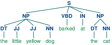
POS tagging
- Goal: assign a lexical category such as noun, verb, adjective, etc. to each word
- needed for lemmatization
- optionally needed for filtering (e.g. nouns only)
- NLTK implements several trained taggers → trained with a large text corpus that is annotated with a certain tagset
- by default:
nltk.pos_tag()for English with Penn Treebank tagset
example = ['The', 'little', 'yellow', 'dog', 'barked', 'loudly', 'at', 'the', 'cat', '.']
nltk.pos_tag(example)    # with default tagset (Penn Treebank)
nltk.pos_tag(example, tagset='universal') # with universal tagset
For German?
- see this blog post
- not implemented in NLTK by default
- with pattern package: ~84% accuracy
- custom tagger for German by Philipp Nolte can be trained with Univ. of Stuttgart's TIGER corpus (uses STTS tagset) → about 96% accuracy
# load a pre-trained german tagger based on ClassifierBasedGermanTagger by Philipp Nolte
import pickle
with open('pos_tagger_german.pickle', 'rb') as f:
    ger_tagger = pickle.load(f)

ger_tagger.tag(['Der', 'kleine', 'gelbe', 'Hund', '.'])
# let's tag our corpus!
tagged_tokens = {}
for doc_label, doc_tok in tokens.items():
    tagged_tokens[doc_label] = ger_tagger.tag(doc_tok)

tagged_tokens['spon2']
Ready for lemmatization
- recap:
- no freely available lemmatizer for German
- partly implemented in pattern → ~74% accuracy with TIGER corpus
- improved lemmatizer germalemma (see this blog post) achieves ~84% accuracy
from germalemma import GermaLemma

lemmatizer = GermaLemma()
lemmatizer.find_lemma('beschuldigt', 'VVFIN')
# let's lemmatize our corpus
tmp_tokens = {}
for doc_label, tok_pos in tagged_tokens.items():
    lemmata_pos = []
    for t, pos in tok_pos:
        try:
            l = lemmatizer.find_lemma(t, pos)
        except ValueError:
            l = t
        lemmata_pos.append((l, pos))
    tmp_tokens[doc_label] = lemmata_pos

tmp_tokens['spon2']
tagged_tokens = tmp_tokens
Final normalization steps
- transform lowercase
- remove special characters
- remove stopwords
stopwords = nltk.corpus.stopwords.words('german') + ['mehr', 'wegen']  # add more words
del_chars = str.maketrans('', '', string.punctuation + '–')   # add another character "–"

tmp_tokens = {}
for doc_label, tok_pos in tagged_tokens.items():
    tok_pos = [(t.lower(), pos) for t, pos in tok_pos]   # to lowercase
    tok_pos = [(t.translate(del_chars), pos) for t, pos in tok_pos]   # remove special char.
    tok_pos = [(t, pos) for t, pos in tok_pos   # remove empty tokens and stopwords
               if t and t not in stopwords]
    tmp_tokens[doc_label] = tok_pos

print('Old:', [x[0] for x in tagged_tokens['spon1']])
print('New:', [x[0] for x in tmp_tokens['spon1']])
tagged_tokens = tmp_tokens
Filtering by POS tag
→ filter words by lexical categories, e.g. only nouns:
[(t, pos) for t, pos in tagged_tokens['spon1']
          if pos.startswith('N')]
Text normalization summary
- many steps from raw input text to normalized tokens
- tokenization
- expand compound words
- POS tagging
- lemmatization
- lower-case transformation
- removing special characters
- removing stopwords </small>
- each step involves decisions that highly effect further analyses
Reproducibility is important!
- document each step
- provide scripts (with code comments) and data with your publication
from pprint import pprint
pprint(tagged_tokens)
Recommended Python packages for text preprocessing
- NLTK – stable but slow
- pattern – many language models but some of them only with low accuracy, Python 2.7 only
- spacy – language models for English and partly for German and French
- SyntaxNet – many language models but difficult to install, Python 2.7 only
- Stanford CoreNLP – many language models but requires Java
Feature Extraction
Features are derived values from our complex data. They should measure certain distinctive properties of our data in order to achieve dimensionality reduction. For each observation a feature vector is created (usually with numerical or categorical values) → Vector Space Model.
Example: A feature vector consisting of three features:
- Token length
- Number of vowels
- Number of consonants
observations = [
    'welcome', 'bienvenue', 'willkommen', 'privetstvie',
]
vowels = list('AEIOUaeiou')
features = []
for obs in observations:
    n_tok = len(obs)
    n_vow = sum([c in vowels for c in obs])
    features.append((n_tok, n_vow, n_tok - n_vow))
list(zip(observations, features))
For linguists, these features might already be interesting. Using machine learning, it might be possible to detect which language a word comes from.
Choosing the right properties for your features greatly depends on want you want to analyse / which methods you want to use → own discipline "Feature engineering"
We will concentrate on Term vector models:
- in a corpus $C$ we have a set of $n$ documents[1] $D_1, D_2, \dots, D_n$ containing terms[2] $t$
- all unique terms in $C$ make up the vocabulary
- each document contains a feature vector $d$ of length $m = N_{vocabulary}$
- a feature vector contains weights $w_i$ of the $i$th term of the vocabulary in that document
$M = \{d_1,d_2, ..., d_n\}$ with $d = \{w_1, w_2, ..., w_m\}$
[1]: Documents are the things you compare. They can be paragraphs, sentences, tweets, articles, etc.
[2]: A.k.a. tokens or words in this context.
Consequences:
- completely based on term weights → weights might denote "importance" of terms in a given document
- term weights usually derived from term frequency
- does generally not take into account: word order, grammar/syntactic structure → information how words relate to each other in a document is lost
- useful for:
- Text classification (Spam/Not Spam, categories, language)
- Summarization / topic discovery
- Text similarity / clustering
- not useful for:
- Semantic and Sentiment Analysis
Bag-of-Words (BoW) model
- simple but powerful model
- features are absolute term counts
- basis for:
- Topic Modeling with Latent Dirichlet Allocation (LDA) via Gibbs sampling
- Text classification with Naive Bayes, Support Vector Machines
- Document similarity
- Document clustering
- ...
Example:
\begin{equation*} C = \{D_1, D_2, D_3\} \\ D_1=\{simple, yet, beautiful, example\} \\ D_2=\{beautiful, beautiful, flowers\} \\ D_3=\{example, after, example\} \end{equation*}| document | simple | yet | beautiful | example | flowers | after |
|---|---|---|---|---|---|---|
| $D_1$ | 1 | 1 | 1 | 1 | 0 | 0 |
| $D_2$ | 0 | 0 | 2 | 0 | 1 | 0 |
| $D_3$ | 0 | 0 | 0 | 2 | 0 | 1 |
from collections import Counter

example_data = ['a', 'b', 'c', 'b', 'b', 'a']
example_counter = Counter(example_data)
example_counter
example_counter.update(['c', 'a', 'a', 'a'])
example_counter
Our normalized tokens with their POS tags are still in the variable tagged_tokens:
pprint(tagged_tokens)
documents = {doc_label: [t for t, _ in tok_pos]   # dismiss the POS tag
             for doc_label, tok_pos in tagged_tokens.items()}
1. Count the tokens for each document:
counts = {doc_label: Counter(tok) for doc_label, tok in documents.items()}
print('tokens:', documents['spon1'])
print('counts:', list(counts['spon1'].items()))
2. extract the vocabulary (set of unique terms in all documents):
vocab = set()
for counter in counts.values():
    vocab |= set(counter.keys())   # set union of unique tokens per document

vocab = sorted(list(vocab))  # sorting here only for better display later
vocab   # => becomes columns of BoW matrix
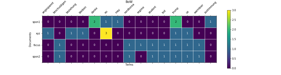
3. Create the BoW matrix:
# create Bag of Words matrix: rows are documents, columns are vocabulary words (unique tokens)
bow = []
for counter in counts.values():  # iterate through each document counter instance
    # make a list that contains the term count of each term in this document
    # if a term of the vocab. does not exist in this document, set it to 0 (default value of .get())
    bow_row = [counter.get(term, 0) for term in vocab]
    bow.append(bow_row)
bow
doc_labels = list(counts.keys())   # => becomes rows of BoW matrix
doc_labels
from utils import plot_heatmap

# show a heatmap of the BoW model
print('spon1:', documents['spon1'])
plot_heatmap(bow, xticklabels=vocab, yticklabels=doc_labels, title='BoW', save_to='img/bow.png')

# 1-grams (unigrams):
documents['spon1']
from utils import create_ngrams

# 2-grams (bigrams):
print(create_ngrams(documents['spon1'], n=2))
Bigrams of our tokens:
documents_bigrams = {doc_label: create_ngrams(doc_tok, n=2)
                     for doc_label, doc_tok in documents.items()}
documents_bigrams['spon1']
from utils import create_bow

bow_bi, doc_labels_bi, vocab_bi = create_bow(documents_bigrams)
plot_heatmap(bow_bi, xticklabels=vocab_bi, yticklabels=doc_labels_bi, title='Bigram BoW');

tf-idf
Problem with BoW: Common words that occur often in many documents overshadow more specific (potentially more interesting) words → can be reduced with stopwords → manual effort
tf-idf tries to decrease the weight of words that occur across many documents → lower the weight of common words.
\begin{equation*} tfidf_C(t, D) = tf(t, D) \cdot idf_C(t) \end{equation*}- $tf$ .. term frequency – related to BoW (raw count or proportion for $t$ in $D$)
- $idf$ .. inverse document frequency – measures how common a word $t$ is across all documents in corpus $C$
term frequency
Better to use relative frequencies than absolute counts: We calculate the term count proportions $tf(t, D) = \frac{N_{t,D}}{|D|}$ for a term $t$ in a document $D$. This prevents that documents with many words get higher weights than those with few words.
We need to convert our BoW to a NumPy matrix type for easier calculation.
import numpy as np
raw_counts = np.mat(bow, dtype=float)         # raw counts converted to NumPy matrix
tf = raw_counts / np.sum(raw_counts, axis=1)  # divide by row-wise sums (document lengths) -> proportions
plot_heatmap(tf, xticklabels=vocab, yticklabels=doc_labels, title='tf / BoW', legend=True, save_to='img/tf.png');

idf – inverse document frequency
Different weighting schemes available. We use this one:
\begin{equation} idf_C(t) = log (1+\frac{n}{1+|D \in C : t \in D|}) \end{equation}- $t$ .. a term (a.k.a. token or word)
- $n$ .. number of documents in corpus $C$
$|D \in C : t \in D|$ .. number of documents in which $t$ appears
plus 1 in denominator to avoid division by zero for unknown words, plus 1 in log to avoid negative numbers
def num_term_in_docs(t, docs):
    return sum(t in d for d in docs.values())

num_term_in_docs('eu', documents)
from math import log

# define a function that calculates the inverse document frequency
def idf(t, docs):
    return log(1 + len(docs) / (1+num_term_in_docs(t, docs)))

idf('eu', documents)
idf_row = [idf(t, documents) for t in vocab]
plot_heatmap(np.mat(idf_row), vocab, title="idf(t)", ylabel=None, legend=True);

Create tfidf matrix by converting idf_row to a diagonal matrix and multiplying tf with it:
idf_mat = np.mat(np.diag(idf_row))
tfidf = tf * idf_mat
plot_heatmap(bow, xticklabels=vocab, yticklabels=doc_labels, title='BoW', legend=True, save_to='img/bow.png')
plot_heatmap(tfidf, xticklabels=vocab, yticklabels=doc_labels, title='tf-idf', legend=True, save_to='img/tfidf.png');


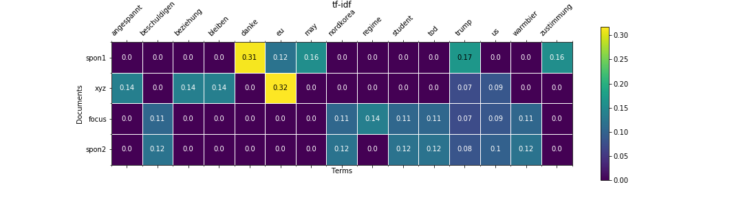
Values in tf-idf matrix are dependent on term frequency (tf) and the inverse document frequency (idf_mat). Tokens that occur in many documents (low idf value) get lower individual tf-idf values.
tf-idf in practice
tf-idf can be used as feature matrix for:
- Topic Modeling (Latent Semantic Indexing (LSI), Non-negative Matrix Factorization (NNMF), Latent Dirichlet Allocation [1])
- Document similarity
- Document clustering
[1]: Depends on implementation – Gibbs sampling based LDA does not work with continuous values, but other implementations (like in [gensim](http://radimrehurek.com/gensim/) based on the [online Variational Bayes](http://papers.nips.cc/paper/3902-online-learning-for-latent-dirichlet-allocation.pdf) approach) seem to [work](https://groups.google.com/forum/#!topic/gensim/OESG1jcaXaQ)