Probabilistic Topic Modeling with LDA
Practical topic modeling: Preparation, evaluation, visualization
Python User Group Workshop
Markus Konrad markus.konrad@wzb.eu
May 17, 2018
Material will be available at: http://dsspace.wzb.eu/pyug/topicmodeling2/
Outline
- Recap:
- Topic Modeling in a nutshell
- Hyperparameters $K$, $\alpha$ and $\beta$
- A topic model for the parliamentary debates of the 18th German Bundestag
- Data overview
- Data preparation
- Model evaluation and selection with model quality metrics
- Visualization
- Some results from the topic model
Recap
What is Topic Modeling?
Topic modeling is an unsupervised machine learning method to discover abstract topics within a collection of unlabelled documents.
Each collection of documents (corpus) contains a "latent" or "hidden" structure of topics. Some topics are more prominent in the whole corpus, some less. In each document there are multiple topics covered, each to a different amount.
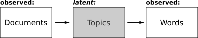
The latent variable $z$ describes the topic structure, as each word of each document is thought to be implicitly assigned to a topic.
The LDA topic model
General idea: each document is generated from a mixture of topics and each of those topics is a mixture of words
LDA stands for Latent Dirichlet Allocation, which can be interpreted as (Tufts 2018):
- topic structures in a document are latent meaning they are hidden structures in the text
- the Dirichlet distribution determines the mixture proportions of the topics in the documents and the words in each topic
- Allocation of words to a given topic
The LDA topic model – Assumptions
- order of words in documents does not matter → "bag of words" model
- order of documents* in a corpus does not matter
- number of topics $K$ is known (has to be set in advance)
* documents can be anything (news articles, scientific articles, books, chapters of books, paragraphs, etc.)
The LDA topic model
An LDA topic model (i.e. its "mixtures") can be described by two distributions:
- a topic-word distribution $\phi$: each topic has a distribution over a fixed vocabulary of $N$ words
- a document-topic distribution $\theta$: each document has a distribution over a fixed number of topics $K$
topic-word distribution $\phi$
What are the topics that appear in the corpus? Which words are prominent in which topics?
Each topic has a distribution over all words in the corpus (vocabulary):
| topic | russia | putin | soccer | bank | finance | possible interpretation |
|---|---|---|---|---|---|---|
| topic 1 | 0.4 | 0.4 | 0.0 | 0.1 | 0.1 | russian politics |
| topic 2 | 0.3 | 0.0 | 0.6 | 0.1 | 0.0 | soccer in russia |
| topic 3 | 0.2 | 0.0 | 0.0 | 0.4 | 0.4 | russian economy |
- $K$ (num. of topics) distributions across $W$ unique words
- topics are a mixture of words → have different weights on words
- topics are abstract – interpretation by examining the distribution
document-topic distribution $\theta$
Which topics appear in which documents?
Each document has a different distribution over all topics:
| document | topic 1 | topic 2 | topic 3 | possible interpretation |
|---|---|---|---|---|
| doc. 1 | 0.0 | 0.3 | 0.7 | mostly about soccer and russian economy |
| doc. 2 | 0.9 | 0.0 | 0.1 | russian politics and a bit of economy |
| doc. 3 | 0.3 | 0.5 | 0.2 | all three topics |
- $D$ (num. of documents) distributions across $K$ topics
- documents are a mixture of topics, each to a different proportion
How do we estimate $\phi$ and $\theta$?
Either: Expectation-Maximization algorithm – an optimization algorithm (Blei, Ng, Jordan 2003)
Or: Gibbs sampling algorithm – a "random walk" algorithm (Griffiths & Steyvers 2004) with iterative resampling
Hyperparameters in LDA
three parameters specify prior beliefs on the data:
- number of topics $K$ – can be found out with model quality metrics
- concentration parameters $\alpha$ and $\beta$ – sparsity of topics ($\alpha$) and words ($\beta$)
there is not one valid set of parameters; you choose if you want a few (but more general) topics or plenty (but more specific) topics
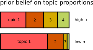
$\alpha$ as prior belief on sparsity of topics in the documents
- when using **high $\alpha$**: each document covers many topics (lower impact of topic sparsity)
- when using **low $\alpha$**: each document covers only few topics (higher impact of topic sparsity)
- $\alpha$ is often set to a fraction of the number of topics $K$, e.g. $\alpha=1/K$
→ with increasing $K$, we expect that each document covers fewer, but more specific topics
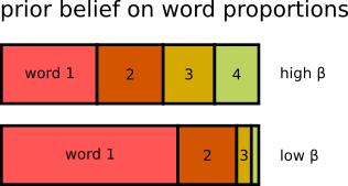
$\beta$ as prior belief on sparsity of words in the topics
- when using **high $\beta$**: each topic consists of many words (lower impact of word sparsity) → more general topics
- when using **low $\beta$**: each topic consists of few words (higher impact of word sparsity) → more specific topics
- $\beta$ can be used to control "granularity" of a topic model
- high $\beta$: fewer topics, more general
- low $\beta$: more topics, more specific
A topic model for the parliamentary debates of the 18th German Bundestag
The data
- proceedings of plenary sessions of the 18th German Bundestag 2013 - 2017
- source: offenesparlament.de
- collects various information about the German Federal Parliament
- project of Open Knowledge Foundation Germany
- raw data: github.com/Datenschule/offenesparlament-data
- information on the data collection and transformation process
Further notes on the data
- data was chosen to act as an example (i.e. not driven by a research question)
- selected as example because:
- data is not trivial to prepare for topic modeling (we'll see why)
- it's in German (more difficult to preprocess than English)
- amount of data is neither too small nor too big (i.e. does not take ages to compute)
- results can be compared with analyses from offenesparlament.de
Characteristics of the data
- CSV files for each plenary session (UTF-8 encoded) with variables:
- sequence: chronological order
- speaker: connected to speaker metadata like age, party, etc.
- top ("Tagesordnungspunkt"): range from very specific ("Bundeswehreinsatz in Südsudan") to very general ("Fragestunde")
- type: categorical "chair", "poi" or "speech" – we only need "speech"
- text: the speakers statement
- missings:
- session #191 was not split into individual speeches (i.e. is a single huge entry)
- amount:
- 243 sessions (excl. #191) with 136,932 speech records in total

The topic modeling cycle
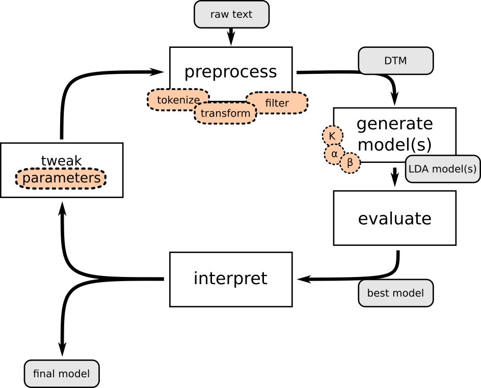
Examine your raw data closely!
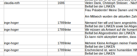
- speeches are divided into several entries (each time when applause, shouts or other calls interrupt the speaker) → should be merged together
- consecutive speech entries with same speaker / same TOP form a speach
- good side-effect: avoids problems with very short speech entries*
- group data by speaker and TOP → concatenate each groups'
textfields
* the length of your individual documents should not be too inbalanced and not too short for Topic Modeling
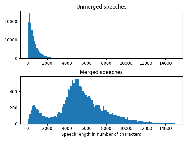
Effect of merging the speeches
Data preparation for Topic Modeling
- LDA works with Bag-of-Words assumption; each document is just a set of word counts → word order does not matter
- textual data must be transformed to Document-Term-Matrix (DTM):
$D_1$: "Regarding the financial situation of Russia, President Putin said ..."
$D_2$: "In the first soccer game, he only sat on the bank ..."
$D_3$: "The conference on banking and finance ..."
| document | russia | putin | soccer | bank | finance | ... |
|---|---|---|---|---|---|---|
| $D_1$ | 3 | 1 | 0 | 1 | 2 | ... |
| $D_2$ | 0 | 0 | 2 | 1 | 0 | ... |
| $D_3$ | 0 | 0 | 0 | 2 | 4 | ... |
Text preprocessing pipeline
Example: Herr Schröder, Sie hatten das Stichwort „Sportgroßveranstaltungen“ bemüht. Dazu sage ich...
| Step | Method | Output |
|---|---|---|
| 1 | tokenize | [Herr / Schröder / , / Sie / hatten / das / Stichwort / „Sportgroßveranstaltungen / “ / bemüht / . / Dazu / sage / ich / ...] |
| 2 | POS tagging | [Herr – NN / Schröder – NE / , – $ / Sie – PPER / hatten – VAFIN / ...] |
| 3 | lemmatization | [Herr / Schröder / , / Sie / haben / das / Stichwort / „Sportgroßveranstaltungen / “ / bemühen / . / Dazu / sagen / ich / ...] |
| 4 | to lower case | [herr / schröder / , / sie / haben / das / stichwort / „sportgroßveranstaltungen / “ / bemühen / . / dazu / sagen / ich / ...] |
Text preprocessing pipeline ... continued
| Step | Method | Output |
|---|---|---|
| 5 | remove special characters | [herr / schröder / / sie / haben / das / stichwort / sportgroßveranstaltungen / / bemühen / / dazu / sagen / ich / ...] |
| 6 | remove stopwords and empty tokens | [herr / schröder / stichwort / sportgroßveranstaltungen / bemühen / sagen / ...] |
| 7 | remove tokens that appear in more than 90% of the documents | [herr / schröder / stichwort / sportgroßveranstaltungen / bemühen / ...] |
| 8 | remove tokens that appear in less than 4 documents | [herr / schröder / stichwort / sportgroßveranstaltungen / bemühen / ...] |
→ finally, generate DTM as input for topic modeling algorithm
DTM from the merged speeches data
- 15,733 rows (i.e. speeches → documents)
- 47,847 columns (i.e. unique words → vocabulary)
- 5,680,918 tokens
- saved as sparse matrix:
- only values $\ne 0$ are stored
- decreases memory usage drastically (from ~2.8 GB to ~50 MB in this example)
Exploring the parameter space
- ready to use topic modeling with LDA now
- how to set the parameters $K$ (number of topics), $\alpha$ and $\beta$?
- generate several models with different parameters values
- use model evaluation metrics to find out the "best" models
- interpret, iterate (see topic modeling cycle)
Excursion: Model evaluation
Model evaluation measures
Human-in-the-loop methods
- word intrusion (randomly replace a word in the list of top words for a topic)
- topic intrusion (randomly replace a topic in the list of top topics for a document)
→ see if domain expert can spot the intruder
→ if topics are coherent, intruders should be spotted easily
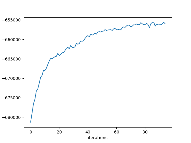
1. Model likelihood
- probability of the model given the data (logarithmic for mathematical reasons)
- theoretic measure of how well the Gibbs sampling process estimated the expected distributions
- does not use held-out data
- calculated each $n$ steps during Gibbs sampling → check for convergence during the Gibbs sampling process
2. Probability of held-out data
- usual approach for supervised machine learning (labelled data!), but harder for unsupervised learning
- evaluate how well trained model predicts test data
- split data into training and test sets
- learn model from training data only; evaluate with test data
- lots of approaches and detailed choices, e.g.:
- how to split data? hold out whole documents or words in documents ("document completion")?
- how to compare training and test outcomes?
- see Wallach et al. 2009, Buntine 2009
- again: does often not correlate with human judgement (Chang et al. 2009)
3. Information theoretic measures
→ which properties should "ideal" posterior distributions $\phi$ and $\theta$ have?
Cao et al. 2009
- uses pair-wise cosine similarity between all topics in topic-word distribution $\phi$
- assumption: good models produce topics that are dissimilar to each other → the lower the cosine similarity, the better the model
- criticism: only takes $\phi$ distribution into account
3. Information theoretic measures
Arun et al. 2010
- symmetric Kullback-Leibler divergence "of salient distributions [...] derived from [$\theta$ and $\phi$]" → takes both distributions into account
- topics should be "well separated" (as with Cao) but also adds penalty for too many "topic splits"
- implemented also in R package
ldatuning
4. Model coherence (Mimno et al. 2011)
- used "expert-driven topic annotation study"
- developed "coherence metric" that correlates with expert opinion
- only relies on "word co-occurrence statistics [...] from the corpus" → no external validation data required
- two use cases: 1) identify individual "bad" topics; 2) measure overall model quality
- lots of extensions to the suggested metric (for an overview see Röder et al. 2015)
Back to the parliamentary debates...
Parameters to evaluate
- three sets of $\alpha$ and $\beta$ parameters:
- "fine": $\alpha=1/K$; $\beta=0.01$
- "medium": $\alpha=10/K$; $\beta=0.1$
- "coarse": $\alpha=50/K$; $\beta=0.5$
- varying $K \in \{20, 30, ..., 100, 120, ..., 200, 250, ..., 500\}$
- number of Gibbs sampling iterations: 1,500 (checked for convergence)
- results in 60 evaluations to be computed (fits well on theia machine w/ 64 CPUs)
Software
- evaluation using metrics implemented in tmtoolkit
- Arun 2010, Cao et al. 2009, coherence (Mimno et al. 2011 and Röder et al. 2015), Griffiths 2004
- runs evaluation in parallel on theia (cluster machine at WZB w/ 64 CPUs)
- took around 3 days to compute
- more metrics could be used (e.g. cross validation w/ held-out documents) but this would take even longer
- similar package for R: ldatuning*
*not sure if computations are done in parallel
Results
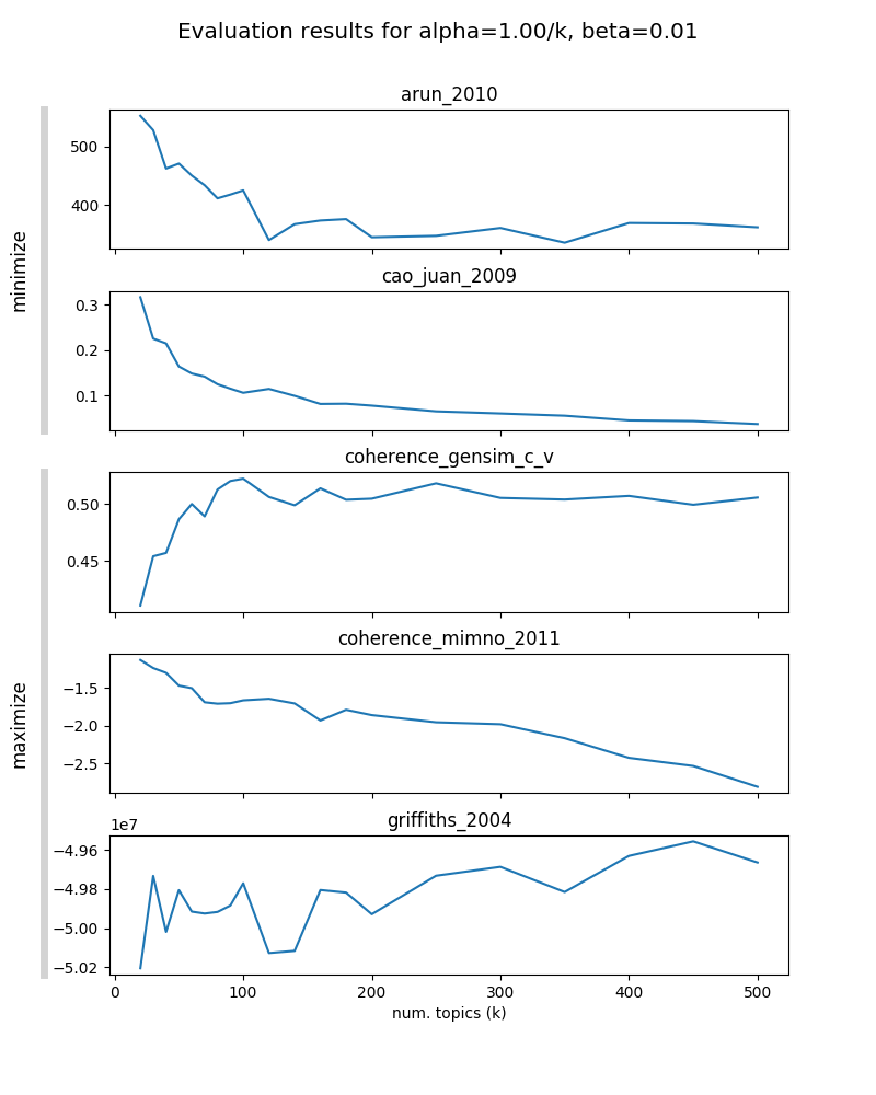
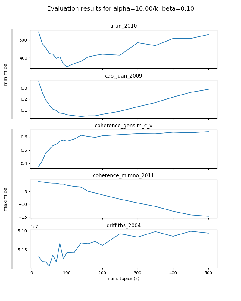
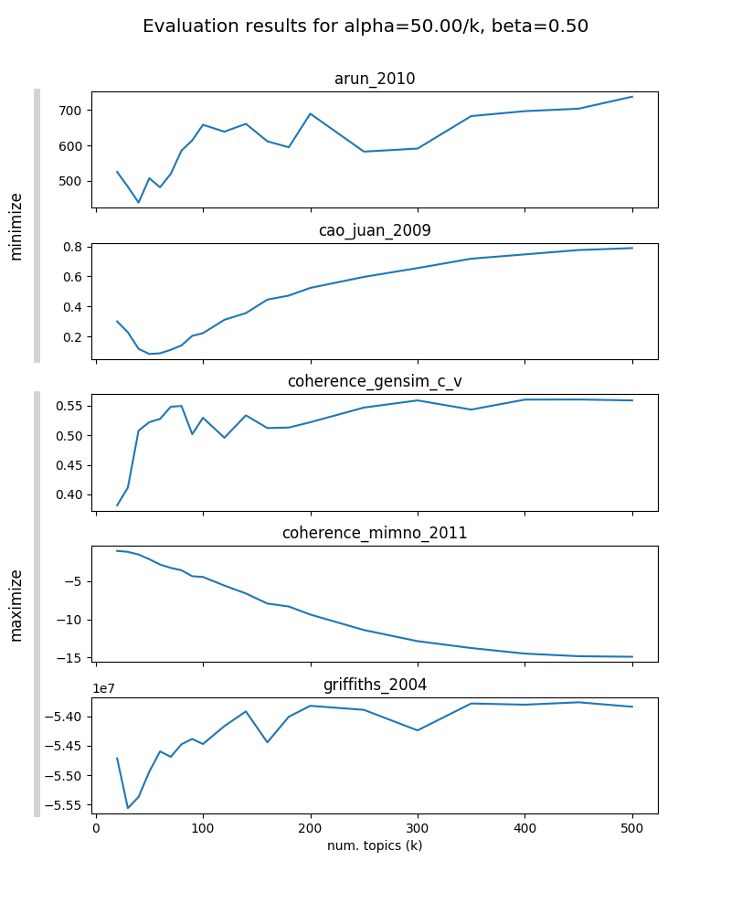
Model selection
- not all metrics seem informative
- with increasing $\beta$, optimal $K$ is decreasing in most metrics (model is less "granular")
- choose "medium granularity" model with $\alpha=10/K$; $\beta=0.1$ and $K=130$
Model inspection – some helpful tools
- summary outputs (e.g. listings with top words per topic / most probable topics per document)
- word saliency and distinctiveness (Chuang et al. 2012)
- helpful to identify very common words (least distinctive words)
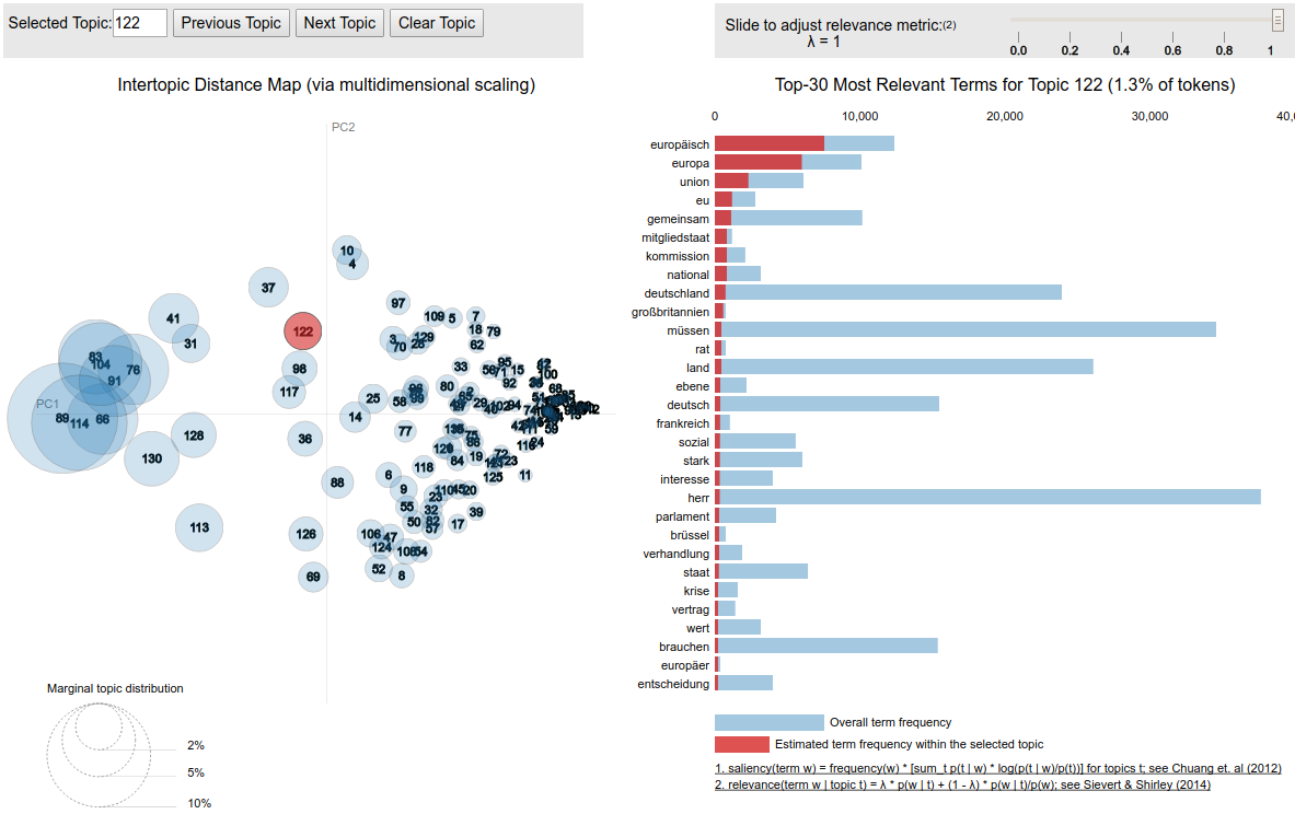
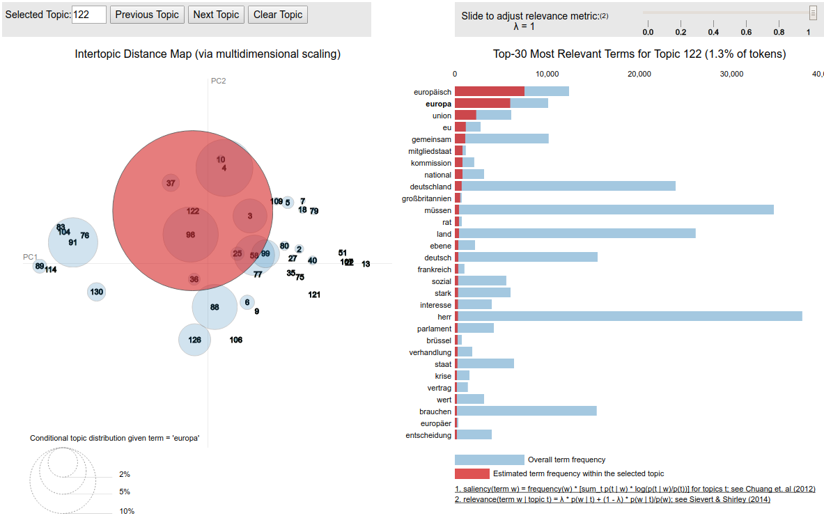
- topic-word relevance (Sievert/Shirley 2014)
- helpful to weaken the weight of very common words in topics
- PyLDAVis (R: LDAVis) (Sievert/Shirley 2014)
- use model coherence metrics to identify incoherent topics
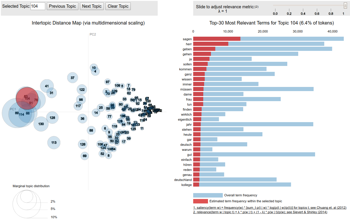
Problems with first model
- too many very general topics and very general words in topics
- saliency and distinctiveness show large amount of very common words like "herr", "dame", "kollege", "sagen"
- some "mixed" topics
- identified with coherence metric (e.g. topic 60 that mixes "india" and "oktoberfest")
Actions for second iteration:
→ add more words to stopword list
→ remove salutatory addresses ("Herr Präsident! Sehr geehrte Kolleginnen und Kollegen! Meine Damen und Herren! ...")
A revised model
- preprocessing revised, evaluation re-run
- 3 days later: similar evaluation results → same parameters chosen ($\alpha=10/K$; $\beta=0.1$ and $K=130$)
Model inspection results
- less amount of too general topics and words
- still ~ 10–20 uninformative topics (incoherent and/or too general)
→ either further tuning or ignore topics that are identified as uninformative
Some results from the generated topic model
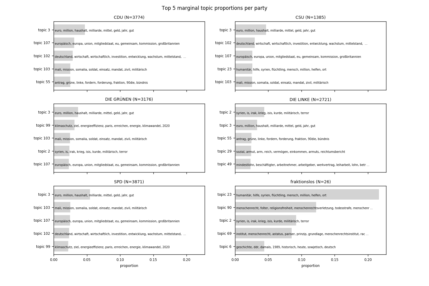
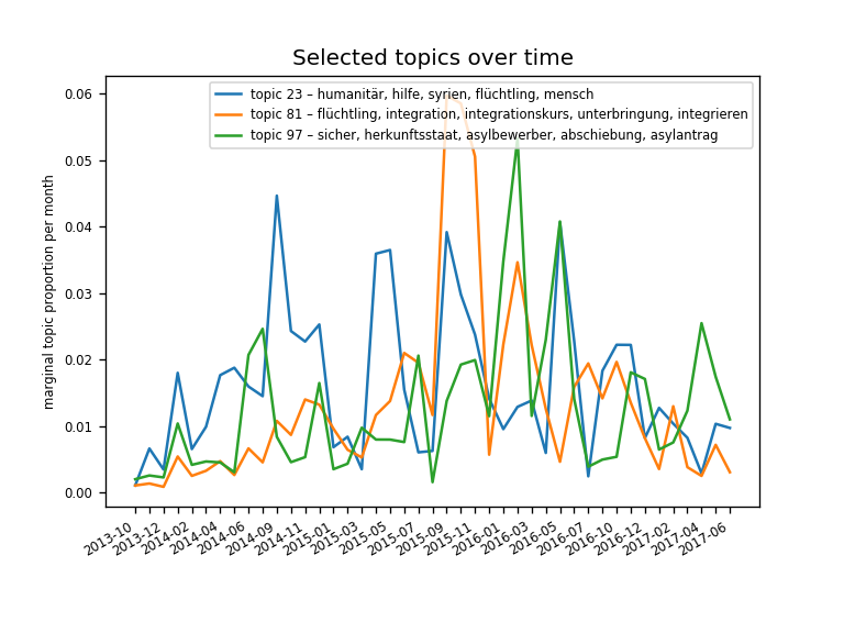
Source code available at: https://github.com/WZBSocialScienceCenter/tm_bundestag
References
- Arun et al. 2010: On Finding the Natural Nurober of Topics with Latent Dirichlet Allocation: Some Observations
- Buntine 2009: Estimating Likelihoods for Topic Models
- Cao et al. 2009: A density-based method for adaptive LDA model selection
- Chang et al. 2009: Reading Tea Leaves: How Humans Interpret Topic Models
- Chuang et al. 2012: Termite: Visualization techniques for assessing textual topic models
- Griffiths/Steyvers 2004: Finding Scientific Topics
- Mimno et al. 2011: Optimizing Semantic Coherence in Topic Models
- Röder et al. 2015: Exploring the space of topic coherence measures
- Sievert/Shirley 2014: LDAvis: A method for visualizing and interpreting topics
- Tufts 2018: The Little Book of LDA
- Wallach et al. 2009: Evaluation Methods for Topic Models </small>